The Output Sheet From the Simulation
The output sheet from the simulation is a "live spreadsheet." You can edit the formulas that are on the sheet in order to change the summary values from the simulation and you can also add new ones if you wish.
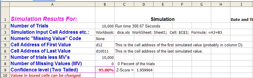
Part I The upper left hand corner of the sheet:
This area of the spreadsheet supplies the constants of the output sheet. Notice that the number of trials is given along with the cell that this sheet is keeping track of. Notice that in this case it is cell C3 or $C$3 from Sheet1. The formula in that cell is the sum of cell A3 + B3. This is the example described in Creating a Simulation Spreadsheet and represents the sum of two die being tossed in cell A3 and B3.
If a non-standard missing value code {i.e. other than the Excel function =NA()} i would be shown in cell B4. The next two cell gives the starting and ending addresses of the simulated values. They will start in cel D12 and continue down the column until the number of simulations has been reach. So the ending cell should be 12 + number of run -1, which is D10011. If there were any missing values included in this total the actual number of real values is in cell B8. This value along with number of missing values are computed by using formulas.The formula in cell B7 could also be written =COUNT(D12:D10011) and it would produce exactly the same result as shown. See Formulas Used in the Output Sheet for an explanation.
In any case in cell B7 the number of value are counted using the COUNTF() function and in cell b8 the COUNTIF() function is used to count the MV's.

Notice that these formulas use two feature that common on the output sheet. One is the INDIRECT() function and the other is the is the ISERROR() function. Both are standard Excel functions.
The confidence interval used in the spreadsheet is given in cell B9, the user can change this level and resulting Z score is recomputed in Cell D9. Any formula on the sheet that uses this Z score will also recompute.
Part II The Lower Left Hand Corner
This part of the spreadsheet contains the summary measures of the results. It also shows the start of the individual simulated values. Which for this example go on until row 11001, so only the first 25 rows are shown.
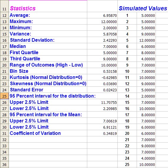
The statistics are formulas. So you can check how each was calculate, and in fact change it if you don't like the results.
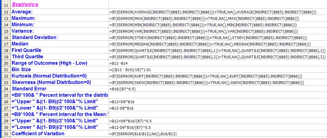
Again the formulas make use of the ISERROR() and INDIRECT() functions in order to calculate many of the values. Some titles use the Excel concatenation operator (&) to create the labels in the first column. One that I change frequently is the Bin Size value. This is discussed below.
If FSrandseq() is used two more lines of output will appear on the output sheet. These will appear as below:
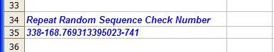
This is a number generated by FinPak to help ensure that you are getting the same repeat of random number for different runs. If you repeat the simulation with different input parameter you show get exactly the same values the next time your run the simulation. If you do not then the same sequence of random numbers was not used. The number after the dash was the seed value, which of course must be same for all runs for which you wish the same random sequence as well as for all occurrences of FSrandseq() in the spreadsheet.
Part III The Frequency Distributions
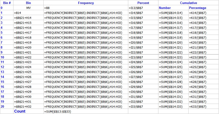
The middle section calculates the frequency distribution in several formats. These use the built-in Excel frequency distribution function to calculate the basic frequency distribution. The other values are calculated from these values.
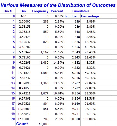
The frequency column is calculated using an array formula, so if you wish to edit it you must edit as a block (See Array Formulas)
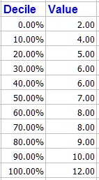
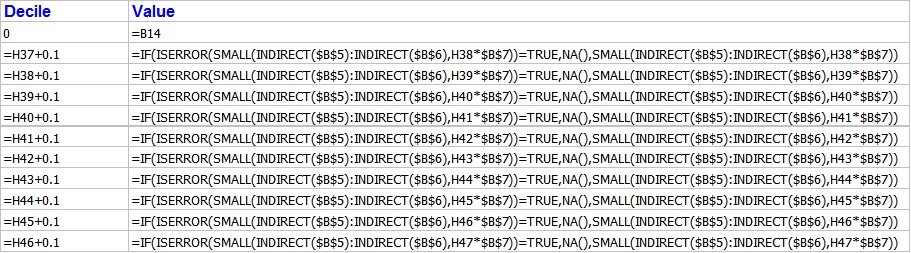
The decile values are also given as shown below these us the Excel SMALL() function to calculate 10% intervals.
Part IV The upper right hand corner
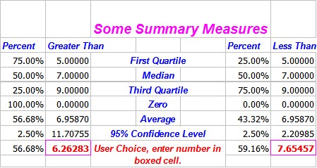
These are given as a summary table. You can change the values in the red boxes to some other limits and the percentages will be computed for those limits. The default limit used in the table is 10% each side of the mean So in this case 56.68% of the values exceed 6.26 and 59.16% of values are less than 7.65.
You can see how these are computed by looking at the formulas on the output sheet, basically the COUNTIF() is used to produce the results.
Part V The Graphs
Each sheet has 4 standard graphs. You can of course create more graphs from the data if you wish.
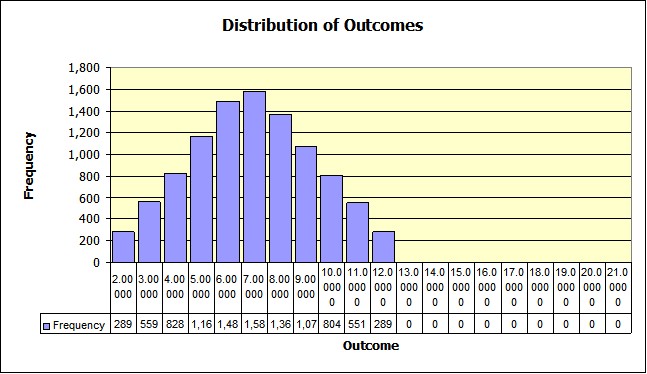
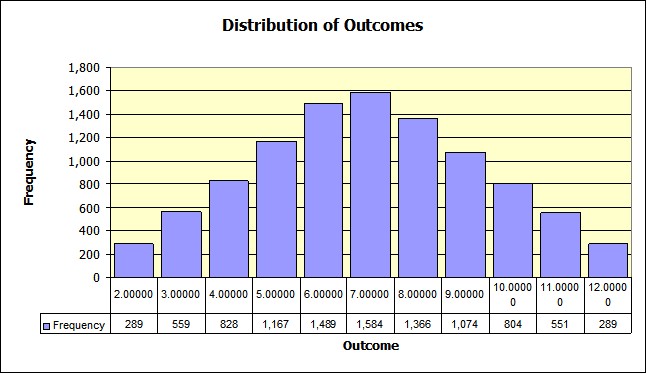
Here is the first graph from the example simulation:
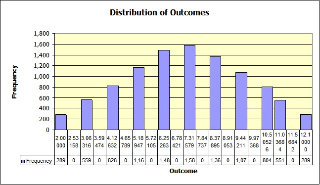
Which is the distribution of the die toss. It gets its data from the frequency distribution using the data from H14:H33 and from I14:I33.
Part VI Changing the Look of the Output
Notice by looking at the distribution and the graph that every other bin is zero. This is because of the number of bins for the frequency distribution is fixed at 20. This makes the bin size: 0.53158 an odd number in this case since the simulation deals with with only whole numbers between 2 and 12. This is one reason a live spreadsheet is handy. You get a better looking graph if you change the bin size to 1. To do this simply type a 1 into the bin size cell which is B21 as show below:
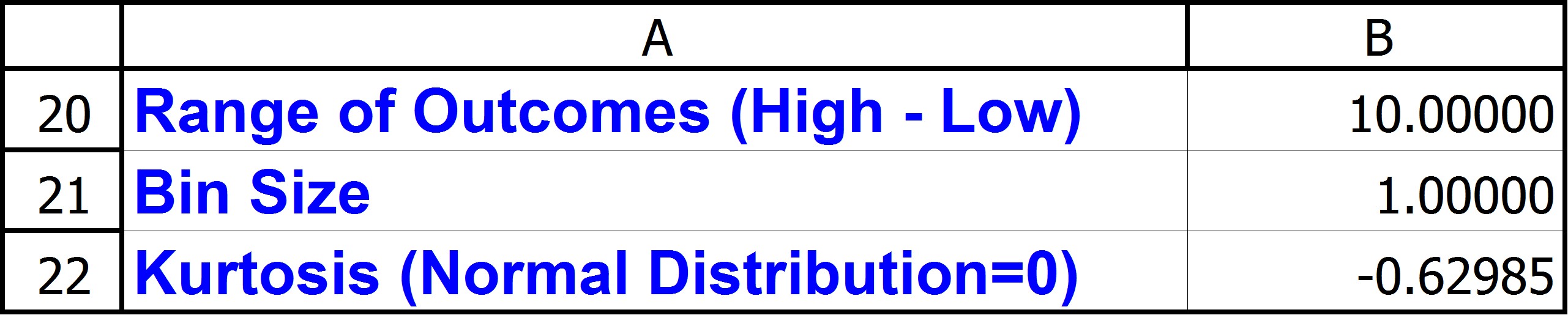
This will remove the formula that computes the bin size and replace it with a constant. You might want to save the spreadsheet before you do this so that you can go back if you wish.
This changes several things on the sheet. For one the frequency distribution now changes as show below:
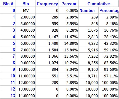
Notice now that only the first 11 bins have values, and bins 12 through 20 are all zero. This changes the graph to the following. Which to the eye look better (I think.).
But it leaves the empty part of the graph to right empty, since it still uses all 20 bins. You can edit this graph (along with others if you wish) to get rid of that also. Right click on the chart's bars, does not matter which one. A box pops up and a
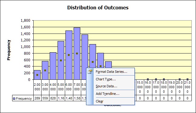
Choose the Source Data option and then choose the Series Tab from the next box and you should be looking at the following.
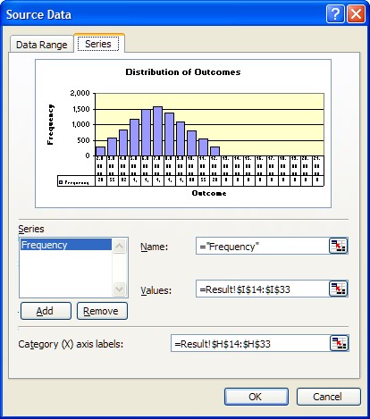
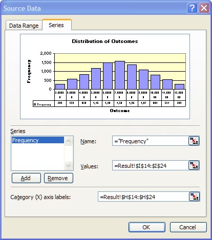
Notice that the values are in I14:I33 (Dollar signs have on impact on the address except to make absolute.) and Category labels in H14:H33. You want to change this to only use the values that are non zero. So click on the navigation box right select the smaller area or edit 33 to read 24, in both cases.
You will see the change immediately in the preview panel above.
Click OK and you will see the graph adjust also. You end up with a nice symmetrical distribution which is what you would expect as shown below
One check of how well the sampling went would be to compute the Chi-Square statistic for the results. It is left as an exercise (the results are consistent with what would expect) all of the necessary sample data to do the calculation is there and available.
Copyright © 2009 Pieter Vandenberg