Error Checking

Formulas Used in the FinPak Output Sheet

If you press <CNTRL> ~ you will see the formulas that are used to compute the various values on the FinPak Output sheet. These value usually depend on the data in column D (the individual results) of the output sheet. Two particular types of formulas are used.

The Indirect Function

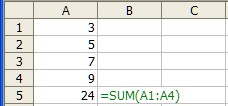
Excel normally expects the function that is being used to point directly to cell addresses. Thus if we want to sum a column of numbers using the sum function such as below:

The sum in Cell A5 uses the Formula: Sum(A1:A4) which say sum the values in that range of cells. An alternative is shown below. In this case the cell addresses of the values we wish to sum are given cell C1 and C2.

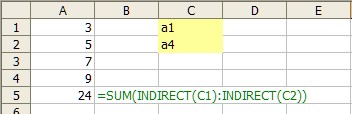
The INDIRECT() function really says sum the values from addresses given in cell C1 to Cell C2. Why bother? It is convenient when you are not sure what values you want to consider and do not wish to modify the formula each time you change your mind.

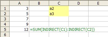
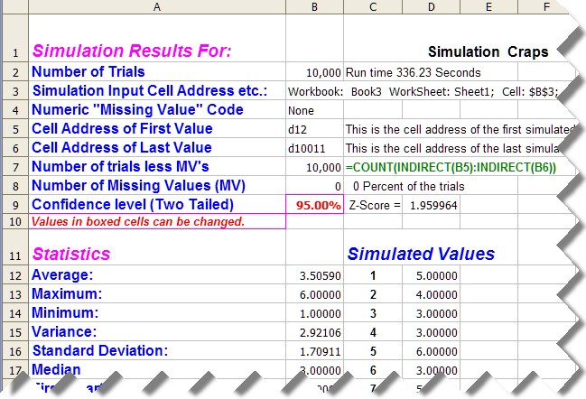
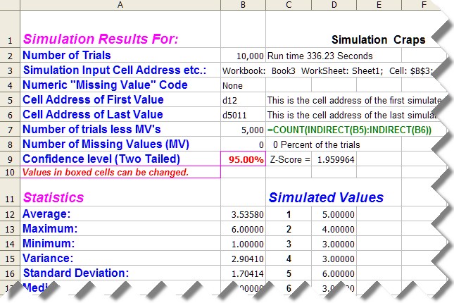
As the example above shows the sum function now adds the values from A2:A3. Thus the formulas on the output sheet are really constant regardless of the number of runs in the simulation and all of the calculations then use the addresses given in cell B5 and B6, which is cell D12 and cell D10011 in the example below (value of cell B7 is determined by using the addresses as the formula in green shows):

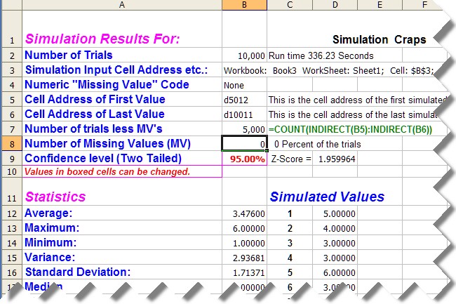
You can put this feature to use. If make a copy of the output sheet you could then change the address in cell B6 to say d5011 and you would get the result below:

This shows that if you had run the simulation for only 5000 runs you would have gotten slightly different results. You could also see what the results would have been had you used the last 5000 runs instead of the first 5000, the results are shown below;

Note that all statistics, frequency and graphs will reflect the addresses cells B5 and B6. If you made copies for each change you could compare the results.

The Error Check

Many of the formulas on the output sheet also perform an error check. In some cases this is a cosmetic issue and in other cases it is essential to the correct functioning of a spreadsheet (See Missing Values.). Below is a look at some of the formulas for used in the output sheet.

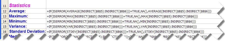
In particular look at the calculation of the average:

=IF(ISERROR(AVERAGE(INDIRECT($B$5):INDIRECT($B$6)))=TRUE,NA(),AVERAGE(INDIRECT($B$5):INDIRECT($B$6)))

First you notice the green values which are simply the addresses and could be replaced with the actual address as discussed above:

Doing makes the formula look less imposing:

=IF(ISERROR(AVERAGE(D12:D10011))=TRUE,NA(),AVERAGE(D12:D10011))

Next notice that the blue parts exact repeats, they always will be in these cases. The first part of the formula uses the

ISERROR(AVERAGE(D12:D10011))

to determine if there is an error in trying to calculate the average, if there is ISERROR returns "TRUE" if not it returns "FALSE."

The IF statement tests to see which occurred checking to see if the result was true:

IF(ISERROR(AVERAGE(D12:D10011))=TRUE, DothisifTrue,DothisifFalse)

If the orange part of the formula is True then the result of the IF test is also "TRUE" and it does the first thing (Dothisiftrue) which results in the value in the cell being set to NA(), if the test result is False, meaning there was no error it does the second thing (DothisifFalse),

which is to compute the average which is what the cell will show.

You can see the rest of the functions do the same thing they all test to see if there is an error and return NA() or value if there is not an error.

Concatenation Operator

This spreadsheet feature is really the answer to question: How much is 1 & 1? Answer: 11.

Concatenation simple combines values. It is useful when you want to combine numbers and words. So to get a cell to display the following calculation "=10/100" as "10 percent" you would use the following:

=(10/100)*100 &" Percent"

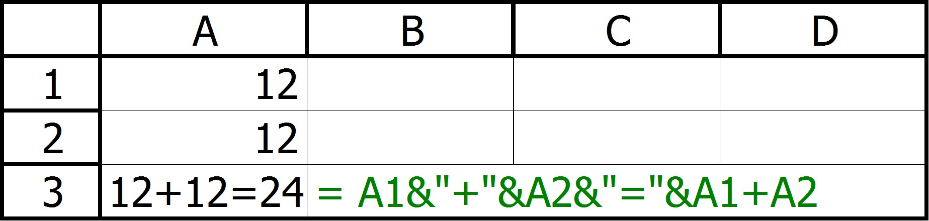
The 10/100 divides; the *100 multiples and moves the decimal place; and the "&" operator appends the Phrase Percent to it. Notice that literals must be enclosed in quotes and in this case a "space" is the first character. Cell addresses can be used and the "&" can be used multiple times as shown in the following example: (Green shows the cell formula in Cell A3)

You will find this technique used in several places in the output sheet.