Using Correlated Random Numbers to Model Variables
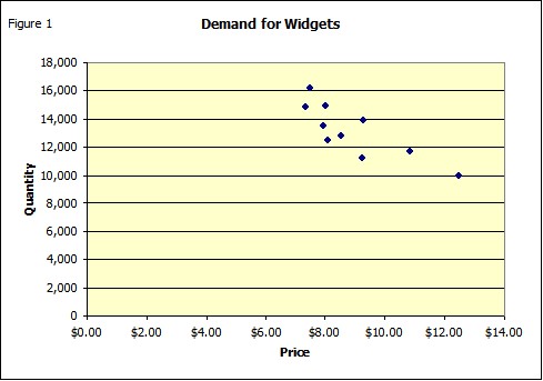
Frequently economic events are not independent. A example is demand for a product (See Explicit Correlation Model). We know from the demand curve that price and quantity are inversely related. Thus in simulating demand it is important to consider this relationship. One way to do this is to use correlated random numbers. In this case you would want to use negatively correlated numbers to estimate demand when prices change. If prices go up demand goes down and vice versa. Figure one shows such an inverse relationship.
If price and quantity were independently modeled this relationship would be lost. In this case using negatively correlated random numbers we select a random number that tends to be from the opposite end of the distribution tor the two variables. Assume that we use a triangle distribution for price with a low of $7.00; a high of $12.00; and a most likely value of $8.00. The value we get in a simulation would depend on the random number. If a low number is returned we get a low price; a high number a high price. The triangle function in FinPak is: FStriangle(low, likely,high, Optional Random number). In this case you want to control the random numbers so use Rand() (or Randseq(seed) to supply the random number.) The following snippet (Table 1) of a spreadsheet shows the setup.
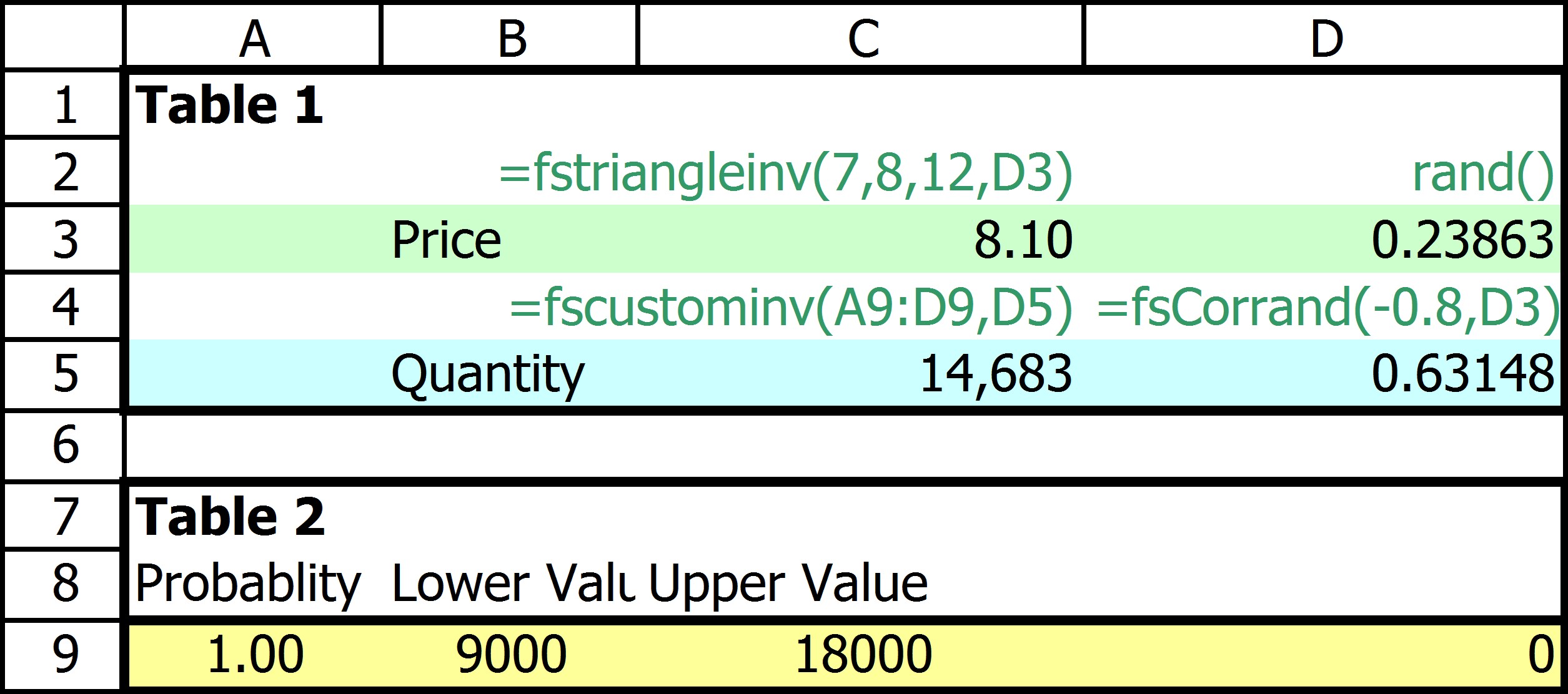
The green row (row 3) is the price simulation. The green values above the cells shows the formulas in the row below. Notice that the function uses the optional input parameter and supplies a random from cell D3. Each time the spread sheet is recalculated a new price is randomly select from the distribution. The corresponding quantity is calculate in row 5 of the spreadsheet. Here the quantity is derived from a distribution, created using FinPak's Custom Distribution Function which in this case selects from a uniform distribution with equal chance of any value between 9000 and 18000. The form of the function is shown above the blue line. The function: FScustominv(A9:D9, D5) uses the values in table 2 which defines the distribution (See Custom Distribution Function for an explanation.) It also uses the value in D5 which is a random number that is negatively correlated (-.80) with the random number (D3) used to estimate the price. The function in D5 is FSCorrand(Correlation Coefficient, Correlated Number) .
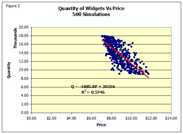
The result is that when price is low (low random number in D3), quantity will tend (correlation =-.80) to be from the high end of quantity distribution and vice versa. Figure 2 shows the result from 500 simulations. It also shows the implicit demand function that resulted from the simulation. It shows the expected inverse relationship, the correlation coefficient given the R2 is -.758. (For 1000 simulations it was -.77, so as the sample size increase the results get closer to -.80.)
More complicated correlations can also be modeled with FinPak with the multiple correlation function. See the discussion of FSMulticorr().
Copyright © 2009 Pieter Vandenberg