Custom Functions

Custom Distribution Function: FScustominv()

FScustominv(Input Matrix,Optional Random Number)

If the available built in functions do not meet your requirements you can supply a custom function. It allows the user to create just about any distribution that can be described. The Fscustominv() function expects the inputs to be in a particular format. There are two inputs to the function, the first is required and the second is an optional random number. This allows the user to control the random numbers used by the function which is convenient in certain cases.

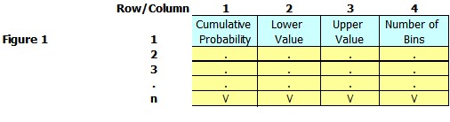
The first input is a table describing the custom function's values. It has the following format (Figure 1): This table should describe the cumulative density function for the input values. (Note you can use the input wizard to create the table, it will also create a graph of the function for you and will attempt to do some basic error checking. See: Input Wizard)

There are always four columns of data. The first is the probability (Column 1) the values between the lower and upper values (Columns 2 and 3). The assumption is that probability of any value between the lower and upper values is continuous. Thus in the following case (Figure 2) the probability of a value (x) 10> x < 20 is 20% and is spread equally over the range. Thus in a random draw approximately half way (.1) would return 15, if the random draw was at the bottom of the range it would return 10 and at the upper end it would return a number approaching 20. Of course figure 2 is not sufficient since the sum of all the probabilities must equally exactly one.

Figure 3 shows a complete input matrix. In this case there are only two rows. The matrix can contain as many rows as are necessary to describe the function. Notice that the last line of any input matrix should always end with a probability of one. So in this case the there is an .80 chance of a value between 20 and 50. The function depends on the values of the random input which will be a number between 0 and 1. You can let the function supply the random number or optionally you can supply it

Notice this table says there is a 20% chance of the value being between 10 and 10 and an 80% chance of the value being between 20 and 50. Figure 4 shows some random draws from this distribution.

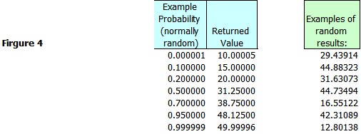
The first two columns show the result for some selected values, while the last columns shows some value randomly selected from the distribution.

The last input column of the matrix has not yet been used. The column allows the user to change the way the values are distributed over the range. Essentially this allows you to distribute the numbers over a discrete set of values. Suppose you are simulating something you know can take on only whole dollar values between $1 and $10. You would set up the input matrix as follows (Figure 5):

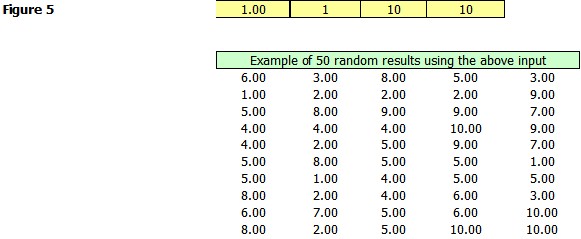
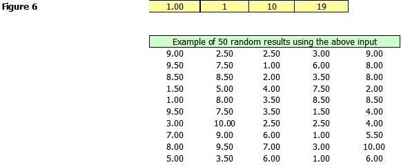
Notice that all of the values are whole numbers between 1 and 10. It is not necessary that they be whole you can divide the interval into as many division as you like (if you leave it blank you are saying essential that there are an infinite number of divisions.) Figure 6 is the setup for 19 bins. Remember that the bin number is inclusive and does not exceed the limits. So in this case the values vary between $1 and $10 in .50 increments.

You can combine both discrete and continuous values in the same matrix. You can also enter exact values for a particularly probability. In the below distribution there is a 50% of a value between 1 and 10 spread over 19 bins, a 20% chance of a value of 12 and a 30% chance of a value between 13 and 15 spread over the entire range equally. Notice that there is no chance of a value between 10 and 12 or a value between 12 and 13. This is a somewhat strange distribution and meant to show the possibilities.

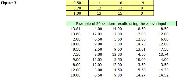
Example Custom Input Distribution:

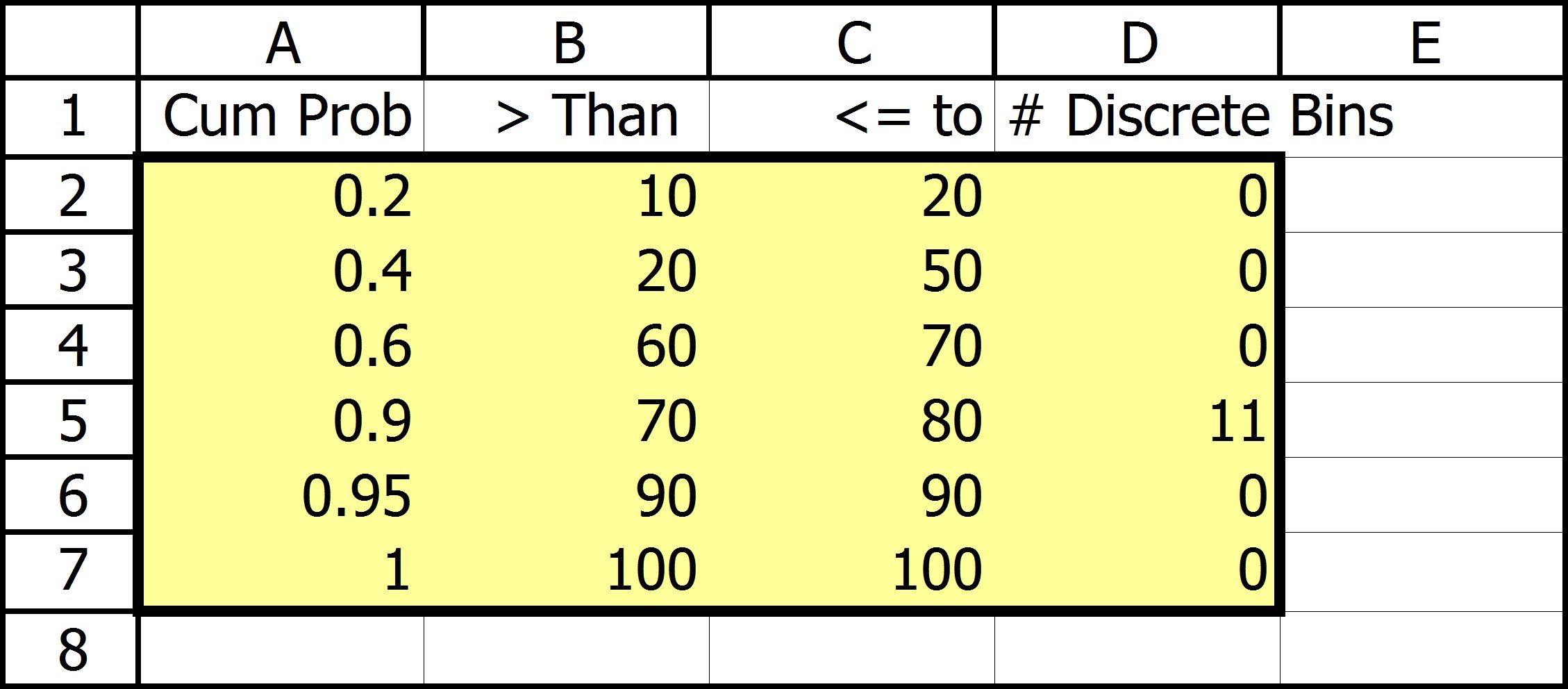
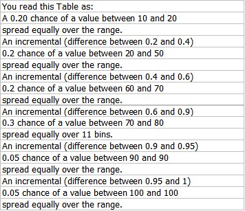
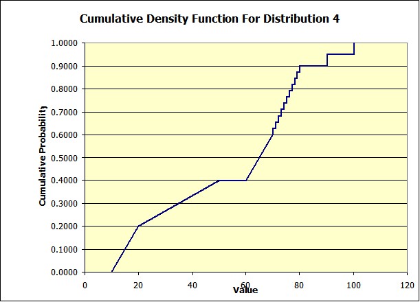
The input distribution can be anything you can dream up. Here is a distribution for a variable that we believe has a 20% chance of a value between 10 and 20; a 20% chance of a value between 20 and 50; a 20% chance of a value between 60 and 70; each of these are spread equally over the ranges. Notice that there is no chance of a value between 60 and 70. Also there is a 20% chance of a value between 70 and 80 spread equally over 11 values, so in this case the value can only take on whole numbers such as 70, 71, 72 . . . 80. Finally there is a 5% of a value of 90 and a 5% chance of a value of 100, nothing in-between.

Here is a graph of the function:

To setup the simulation you would enter the following in a cell:

=fscustominv(A2:D7)

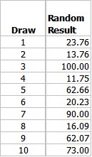
Notice in this case the function will supply the random numbers, since the optional random input was left out. Here are 10 random draws from the distribution:

Also the inputs do not have to come from the same sheet as the simulation. Thus you might have put the input data on a separate sheet called "Distribution 4" in that the case the inputs would have looked like this:

=fscustominv('Distribution 4'!A2:D7)

If you had wanted to add your own random numbers it might have looked like this:

=fscustominv('Distribution 4'!A2:D7, fsrandseq(8712))

Setting up the table is not difficult but if you wish you can use a wizard to build the table it will also create the graph for you. That's in fact where the above graph came from. For information about the wizard click here.