Modelling Correlation

Explicit Model of Correlation

Frequently economic events are not independent. An example is the demand for Widgets. We know from the demand curve that price and quantity are inversely related. Thus in simulating demand it is important to consider this relationship. One way to do this is to use correlated random numbers. In this case you would want to use negatively correlated numbers to estimate demand when prices change. If prices go up demand goes down and vice versa.

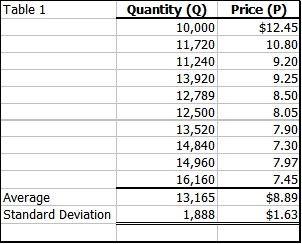
While we can use correlated random number which could build some relationship between the variables of price and quantity it is probably a better idea to specifically model the demand relationship. This sections suggests a way to do that. Table 1 below gives the quantity sold for a given price. (For this example we won't worry about where the firm got this data.)

Having this data allows the firm to estimate the demand function, which tries to explain why the quantity sold varies by using price. There are several way that this can be done in Excel. Table 2 is output from the Data Analysis Regression wizard in Excel (there are several other ways to this in Excel).

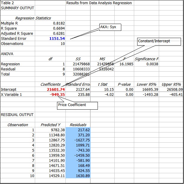
Explaining all of the output is beyond our scope. But there are several useful bits of information presented that are needed. The first is the demand equation (red numbers): Quantity = 21601.74 - 949.35*Price. This equation does a reasonable job of explaining the quantity, but certainly not a complete job. The correlation coefficient is .8182 which indicates that something beside price probably influences demand. Another way to see this is to look at the residuals (blue background), which uses the equation and the given price to back test to see how well the equation fit the data, notice that sometime the equation over estimates and other times it under estimates. The standard deviation of these residuals is called the Standard Error* (the blue number): 1151.54, also known as the standard error of the estimate and frequently abbreviated: Syx. If the residuals were all zero standard error would be zero. The figure below shows that the equation (red) line does not pass through all the points.

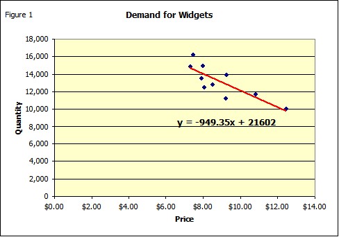
Now it turns out that residuals from a regression are/should be normally distributed with a mean of zero (you can check it) and a standard deviation equal to the standard error (if you check this be sure to correct for the degrees of freedom). If you substitute the prices in Table 1 into the equation you will get the red line in Figure 1 (these numbers are called the Predicted Y in Table 2. Thus given the price there is no uncertainty about the predicted quantity, if you use the equation, since all points fall on a straight line (Figure 2). Of course this does not account for the residuals.

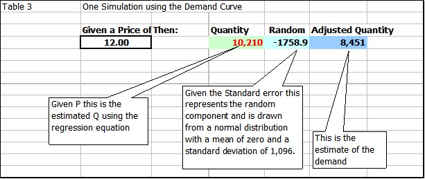
The random component of -1758.9 is estimated using the FSnorminv function in Finpak. FSnorminv returns a normally distributed value given the mean (in this case zero) and standard deviation (in this case 1151.54). Notice that the random component would be recalculated each time the spreadsheet is recalculated. Which means if we used the price of 12.00 again the random value would be different.

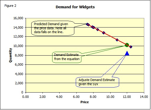
Figure 2 shows the over-all relationship.

The file Simple Project Simulation 1000.xls has a complete example worked out and includes the result for 1000 runs of the simulation.

* Note: The use of Standard Error may not always be the best way to simulate the potential deviation from the expected relationship. It is known that individual estimates of the confidence limits for errors of the dependent variable (Quantity), given an independent variable (Price) maybe biased low. This is particularly true if the independent variable is significantly away from the mean of the values of the independent variable. The correction is to increase the confidence limits for the distance it is away from the mean. (Any statistics book can give you the formula.)