Missing Value Replace

Replace Missing Values (MV's)

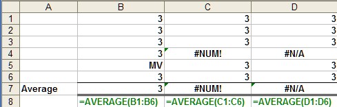
FinPak inserts the literal value MV whenever the simulation results in a non-numeric outcome. Excel Statistical functions ignore an alphabetical value when calculating a value. (The formula used in row 7 is shown in green in row 8.)

Notice that average is calculated for the data in column B, but not for Columns C and D. FinPak replaces the NA() function with the literal "MV" in the output sheet, however this replacement will fail if any other error occurs such as #NUM or #VALUE. The replacement allows the statistical values to be calculated.

What would cause a value not to be numeric. Here is a simple example:

Here are a set of cash flows produced by the simulation of an investment:

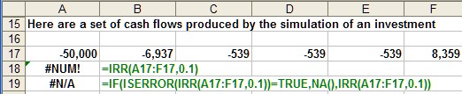
Notice that the attempt to calculate the IRR in cell A18 results in #NUM error. In order to avoid this problem the best way to compute the IRR is to do it as is done in cell A19. In this case the IRR is checked for an error using the ISERROR() function and if an error is present the value is set NA(), if no error is present then the value will be the IRR, as shown below:

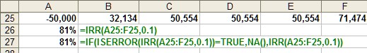
Cells A26 and A27 produce the same result when there is no error. So for simulation you want to capture those errors and you should use cell A27 instead of A26

The above simulation was run 500 times and the MV value came up 11 times. Thus the average IRR and other measure effectively ignored this event. Since the NPV were also simulated it was discovered that every time there was an error the NPV was very negative. This can be seen below:

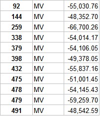
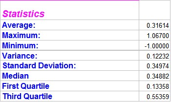
So in this case it may make sense to adjust the values in the IRR spreadsheet by assigning a negative IRR in place of the MV's. Suppose you used -100% (or -1.00)

You click on the Replace MV's button and you are given a warning about make sure you have a back-up copy and then the MV's are replaced.

Note the undo data is stored in the spreadsheet starting in cell AD12. Here is the impact on the summary statistics of this change: