Log Normal Distribution

FSlognorminv(Mean, Standard Deviation, Optional Random Number)

The log normal distribution is ubiquitous in Finance. The most common use of the log normal in finance is to assume that asset prices follow a log normal distribution. The common option pricing models all use this assumption. Excel has a built in log normal distribution functions, in various forms including an inverse function which is what you would likely use in simulation. For ease of use and consistency there is a FinPak function for the log normal inverse that expects as inputs the mean, standard deviation and an optional probability which is a random number between 0 and 1. FinPak will supply the needed random value if you leave it out.

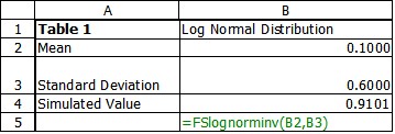
The following would provide a simulation of a normal distribution with a mean of .10 and a standard deviation of .60

=fslognorminv(.10,.60)

Each time the spreadsheet is recalculated a new value is sampled from the distribution. Of course the inputs can be entered as variables as shown in Table 1

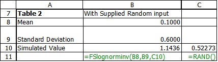
And the user can supply the random number with Rand, or from an alternative source such as FSRandseq if desired. (If you use the native Excel loginv() function you must supply it.)

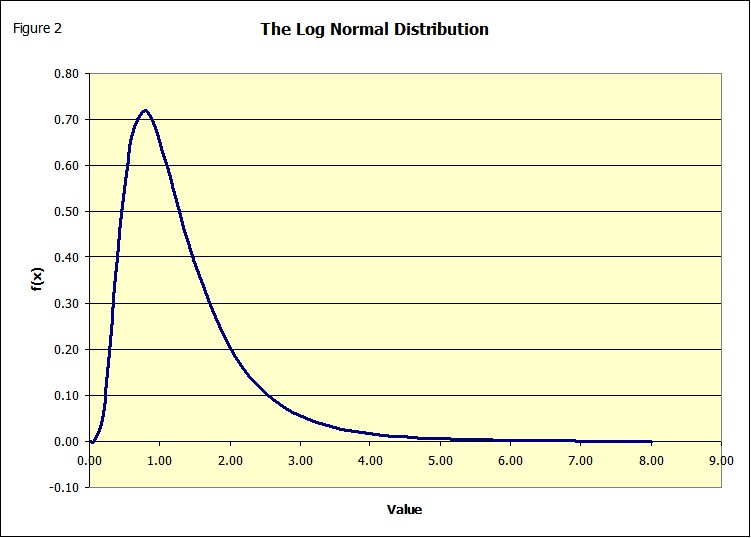
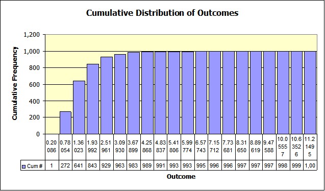
The simulation is drawn from the Cumulative Function (Figure 1), not the familiar Distribution function (Figure 2). These figures were drawn using the theoretical normal distribution function in Excel.

The first point is the result of a random number = .52273, a second run of the simulation produces the second point with a random number = .2381

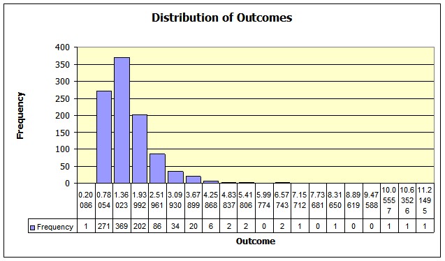
By reading from the X axis we can see the simulated value for the first point is 1.1436(table 2) and the second point has a value of .7208. If you were to simulate this process for a few thousand times how would the result look?

With a large enough number of trial they should look exactly like figures 1 and 2. Figures 3 and 4 show the resulting histograms, for 1000 trials. They would look even closer if the number of trials were increased.