Considerations in Spreadsheet Design

The recommendations below on design of a spreadsheet is somewhat like asking: Who has the best looking spouse? This seems an easy way to start a fight and when you are all done you still haven't answered the question.

A Simple Project: (see the file Simple Project.xls)

The Story: (This project is very simple and does not contain a variety of issues that most projects contain.)

A firm has a new project to produce Widgets which has a required investment of $100,000 and has an expected and a depreciable life of 10 years. The firm expects that it will sell 13,000 Widgets at a price of $9.00 each year. The cost function is $10,000 + $5.00 per unit produced. The investment has a zero expected salvage value and will depreciated using straight line. The tax rate is 40% and the discount rate is 15%.

If you view project analysis as finding the IRR and/or the NPV you can solve this problem in two cells of a spreadsheet.

There is no advantage to using a spreadsheet as a calculator. You might just as well use a calculator. In a mathematical sense the answer is correct. But it is a waste of the spreadsheet's capabilities.

The following design is not much better. It just prints out the cash flows.

A much better design and one that can be analyzed and simulated is the following one:

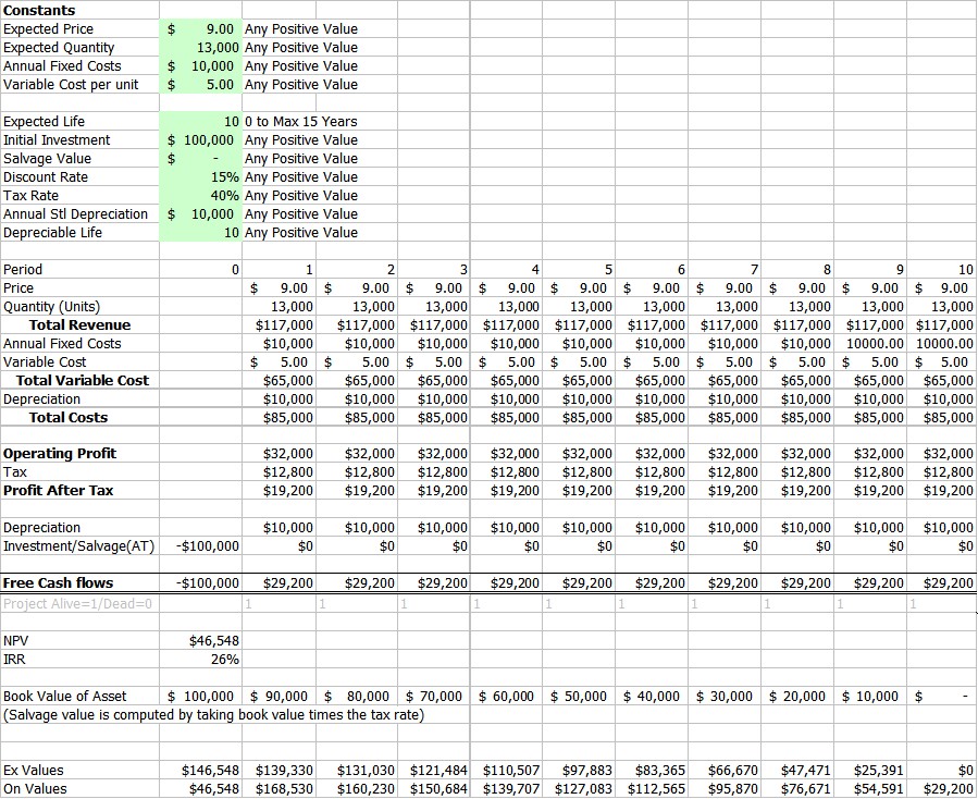
The constants are entered into the spread sheet and Cash flows all refer to the constants. Additional information about the value of the project is supplied (Ex/On Values). The life of the project is treated differently from the life of the depreciable asset. The life of the project can be changed from the expected life. I have assumed for simplicity that it can be done without additional investment. All of the variables in the green box are dynamic and can be changed at will to see the impact on the value of the project. Next to each variable is the allowable range of data values. The limitation on life is caused by the number of columns programmed in. It would require slight modifications to use values beyond those given. (Since the spreadsheet can handle only 256 columns there is an absolute limit.)

Setup this a variety of analysis can now be performed. You can look at the impact on changes in the constants (which in this case are really the assumptions). There are a variety of spreadsheet techniques that could be used. It is also setup to make it fairly easy to simulate the project. What can be learned about the project?

Simulating the Simple Project (see the file Simple Project Simulation.xls)

A Few additions to the Story

This spreadsheet takes the Simple Project a step further, by using simulation to study the characteristics of the project. Remember simulation is not a cure-all for project analysis. It is use in this case since we five variables that interact to produce the cash flows for the project.

These are:

Price, which we assume follows a triangle distribution with:

Lowest: $7.00

Most Likely: $8.00

Highest: $12.00

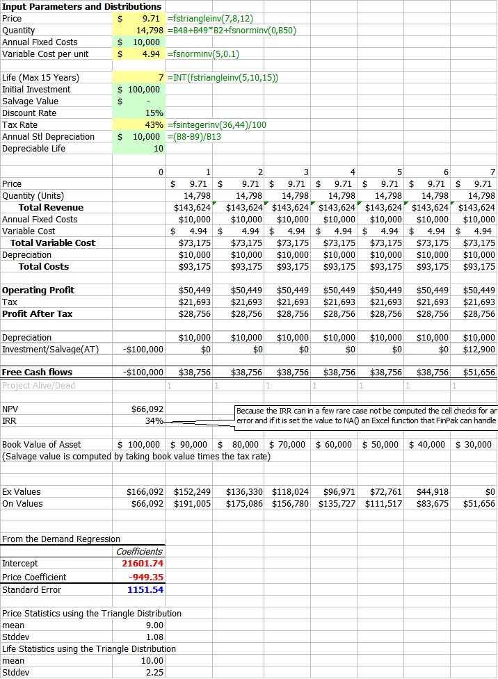
Quantity, which has a demand curve as given by the data in sheet Demand Regression. This data provides a demand curve estimate of Quantity = 21,601.74 - 949.35*Price. Of course being a statistical estimate it does not perfectly explain the actual demand. The Standard Error of the Regression (Syx) is 1151.54 units. We know that regression errors/Residuals are normally distributed with a mean of zero and a standard deviation equal to the standard error. We can use this to simulate the quantity by using the demand curve and the standard error.

Variable Cost, is estimated to be normally distributed with a mean of $5.00 and a standard deviation of $.10, which means the firm is relatively certain about this number. A 95% confidence would indicate a value between $5.20 and $4.80.

Life, of the project is expected to be 10 years. It follows a triangle distribution with:

Lowest: 5 years

Most Likely: 10 years

Highest: 15 Years

Tax rate is estimated to be 40%, with equal chances of a value between 36% and 44%.

The IRR of the project is going to be simulated. While NPV is computed it is not used. Why? Complicated, but to computed it requires the very thing we are trying to find out, what is the risk. If we already knew that we would not need the simulation to compute the NPV.

Below is one run of the simulation. The yellow cells are the values being simulated. The green cells are constants, we could also include those if we so wished. To the right of the yellow cells are the formulas (and therefore the distributions) that are being used to simulate the values. Price and life are triangle distributions; Quantity is determined by the result of a demand regression and normally distributed errors; the variable is normally distributions and the tax rate is equally distributed over a range. Note that it might be better spreadsheet design to move the input parameters with in the functions to a cell and refer to their cell address.

The simulation was run 1000 times and kept track of the IRR and all of the input variables. You can look at the reference file to see the results. Here are some of the statistics for the IRR:

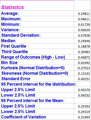
The distribution of IRR's looks like this:

Now the real hard work begins. What can learned from the simulation about the characteristics of this investment?